1 Sistema ng Smart Home Batay sa ZigBee
Sa patuloy na pag-unlad ng teknolohiya ng kompyuter at teknolohiya ng kontrol ng impormasyon, ang mga smart home ay nag-evolve nang mabilis. Ang mga smart home hindi lamang nakakapag-retain ng mga tradisyonal na residential na functions kundi nagbibigay din ito ng convenient na paraan para sa mga user na ma-manage ang mga household devices. Kahit nasa labas pa ng bahay, maaaring remotely monitorin ng mga user ang internal status, na nagpapadali sa energy efficiency management at malaking pagtaas sa quality of life.
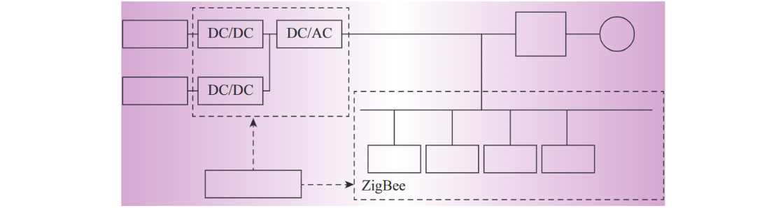
Ang paper na ito ay nag-disenyo ng sistema ng smart home batay sa ZigBee, na binubuo ng tatlong components: home network, home server, at mobile terminal. Ang sistema ay simple, efficient, at highly scalable, na may structure na ipinapakita sa Figure 1.
1 Arkitektura ng Smart Home Batay sa ZigBee
1.1 Home Network
Bilang core foundation, ang home network ay konekta ang controllable loads bilang nodes para sa internal data transmission at multi-energy management. Ang pagpipili ng wireless (ZigBee) sa halip ng wired solutions ay nagpapataas ng flexibility, reliability, at scalability. Ang ZigBee, na batay sa IEEE 802.15.4, ay nag-aalok ng mababang cost, power, at complexity kasama ang mataas na seguridad. Ang mga affordable chips nito ay nagbabawas ng system hardware costs. Ang network ay kinabibilangan:
1.2 Home Server
Ang server ay gumagampan bilang “data-control core” ng sistema, na nag-handle:
1.3 Mobile Terminal
Batay sa Android (Eclipse + Java), ang terminal ay nag-enable:
2 disenyo ng Home Energy Efficiency Management
2.1 System Architecture & Logic
Integrating “smart home + PV + energy storage”, ang sistema ay nagsasama ng efficiency strategies sa server, na nag-form ng “collect → model → optimize” loop:
2.2 Core Components & Collaboration
Key components (PV arrays, batteries, inverters, server, loads) gumagana bilang:
2.3 Load Classification & Scheduling
Loads split into three types for time-of-use pricing-driven scheduling:
Ang server controls shiftable loads via smart sockets, shaving peaks/filling valleys to cut costs and stabilize the grid.
3 Mathematical Model and Control Strategy for Home Energy Efficiency Management
3.1 Mathematical Model for Home Energy Efficiency Management
Upang makamit ang precise home energy efficiency management, kailangang itatag ang mathematical model para sa total electricity cost. Ang paper na ito ay gumagamit ng “daily” control cycle, na pinaghahati ang 24 oras sa n equal time intervals. Sa pamamagitan ng discretizing continuous problems (kapag ang n ay sapat na malaki, bawat interval ay lumapit sa “micro-element,” at ang variables ay maaaring ituring na constant sa loob ng interval). Sa ika-t interval, batay sa dynamic balance ng “home load power, photovoltaic generation power, battery charging/discharging power, at grid interaction power,” ang system power balance equation ay nakuha bilang:

Sa loob ng ika-t time interval, ang power variables ay inilalarawan bilang:
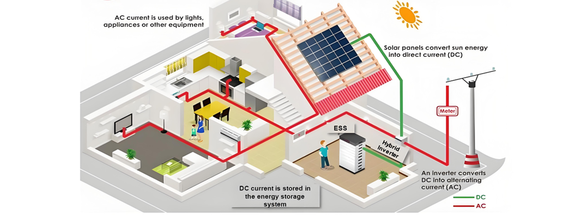
Ang household PV system ay gumagana sa ilalim ng “self-consumption + surplus power grid-feeding” model, kung saan ang sobrang electricity ay nag-generate ng grid-feeding revenue at ang PV generation ay qualified para sa subsidies. Kasama ang time-of-use (TOU) pricing (mas mataas na peak rates, mas mababang off-peak rates), ang total electricity cost ay ina-compute bilang:Total Cost=Grid Purchase Cost−Grid-Feeding Revenue−PV Subsidies
Para sa daily cycle na discretized sa n intervals, ang total cost model ay maaaring lalo pang decomposed sa summation ng interval-specific costs, na precisely adapting sa dynamic pricing scenarios.
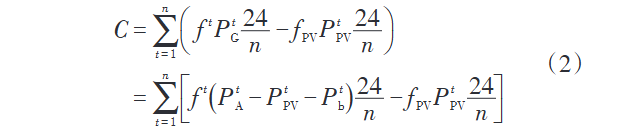
Sa formula: C represents the total daily electricity cost of the household; fPV is the unit price of the photovoltaic power generation subsidy; 24/n is the duration of one time interval.
The expression for \(f^t\) in Formula (2) is

Sa formula: \(f_{\text{C}}^t\) is the electricity price for the user during the t-th time period, which is divided into peak-time electricity price and off-peak electricity price according to different time periods; \(f_{\text{R}}\) is the electricity price for surplus electricity fed into the grid. The values of \(f_{\text{C}}^t\), \(f_{\text{R}}\) and \(f_{\text{PV}}\) at any moment of the day are all known. The total power \(P_{\text{A}}^t\) of the household load is equal to the sum of the power of all shiftable loads and other loads during the t-th time period.

Sa formula: \(P_{\text{L},i}\) is the operating power of the i-th shiftable load; \(T_{\text{L},i}\) is the start-up time of the i-th shiftable load; \(\Delta t_i\) is the operating duration of the i-th shiftable load; \([t_i^s, t_i^e]\) is the range of the start-up time of the i-th shiftable load. \(P_{\text{L},i}\), \(\Delta t_i\), \(t_i^s\) and \(t_i^e\) are all definite values.
The electric power \(P_{\text{else},j}^t\) of other loads is known, while the electric power of shiftable loads changes according to different start-up times, and \(T_{\text{L},i}\) is an undetermined value. When \(T_{\text{L},i}\) is different, the total power \(P_{\text{A}}^t\) of the household load changes accordingly, thus changing the total household electricity cost C.
3.2 Control Strategy
The core goal of home energy efficiency management is maximizing economic benefits, specifically translated into constructing an objective function for "minimizing the total household electricity cost C".
Based on the shiftable load model and combined with the time-of-use pricing mechanism, adjusting the start-up time \(T_{\text{L},i}\) of shiftable loads can dynamically optimize the total household load power curve, reducing the total cost from the perspective of electricity consumption timing.
Coordinated Control Logic for PV and Energy Storage
For photovoltaic (PV) power generation and energy storage batteries, control strategies are formulated for different time periods:
Battery Constraints
It is necessary to simultaneously consider the charging/discharging power limits and capacity restrictions of the battery to constrain its charging and discharging behaviors (specific constraints need to be supplemented with formulas/models, not fully presented in the original text), ensuring equipment safety and system stability.
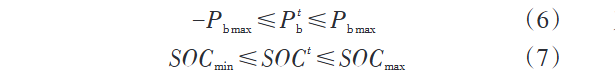
In Formula (6): \(P_{\text{b,max}}\) is the maximum charging/discharging power of the battery; in Formula (7), \(SOC^t\) is the state of charge (SOC) of the battery during the t-th time period; \(SOC_{\text{min}}\) is the minimum value of the battery’s SOC; \(SOC_{\text{max}}\) is the maximum value of the battery’s SOC.
According to the control strategy, optimize and control the charging/discharging power of the energy storage battery. During the peak period \(t \in [t_1, t_2]\), where \(t_1\) is the start time of the electricity peak period and \(t_2\) is the end time of the electricity peak period, the discharge power of the battery is set as

During the off-peak period \(t \in [1, t_1]\), the discharge power of the storage battery is set as

It is necessary to calculate the state of charge (SOC) of the storage battery. The relationship between the state of charge during the charging and discharging process of the storage battery and the charging/discharging power is as follows:
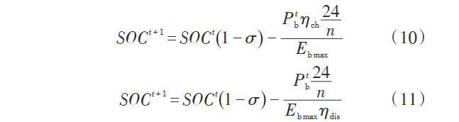
Formula (10) describes the relationship between the storage battery’s SOC and charging power during charging (here \(P_{\text{b}}^t < 0\); Formula (11) describes that during discharging (here \(P_{\text{b}}^t > 0\). \(SOC^{t + 1}\) is the SOC in the \(t + 1\)th period; σ (self-discharge rate, nearly 0% for small time intervals), ηch (charging efficiency), ηdis (discharging efficiency), and \(E_{\text{b,max}}\) (max capacity) are battery parameters. In summary, home energy efficiency optimization aims to minimize total electricity cost by determining shiftable loads’ start times and energy storage charging/discharging power at each moment, stated as:
Objective function

Constraint conditions

4 Case Analysis
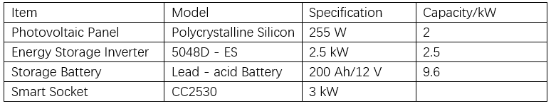
To verify the effectiveness of the proposed home energy efficiency management method, simulations and analyses are conducted using the household electrical equipment of a typical household in Shanghai. The home energy efficiency management system consists of photovoltaic panels, batteries, an inverter, a home server, and household loads. The system configuration parameters are shown in Table 1.
Shanghai implements time-of-use electricity pricing for residential living electricity, with peak hours from 6:00 to 22:00 at 0.617 CNY/kWh, and off-peak hours from 22:00 to 6:00 the next day at 0.307 CNY/kWh. The feed-in tariff for surplus PV electricity is 0.4048 CNY/kWh. Shanghai’s photovoltaic power generation subsidies include a national subsidy of 0.42 CNY/kWh and a local subsidy of 0.4 CNY/kWh, totaling 0.82 CNY/kWh.
Assume that the maximum charging-discharging power of the battery is 1.5 kW; the minimum state of charge (SOC) is set to 0.2, and the maximum is 0.9. The initial SOC \(SOC^1\) of the battery is set to 0.2; the charging-discharging efficiency of the battery is 0.9.
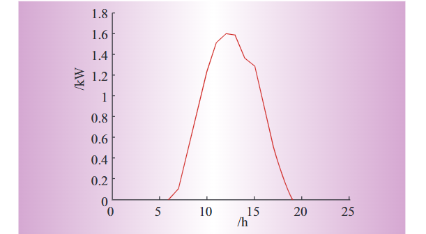
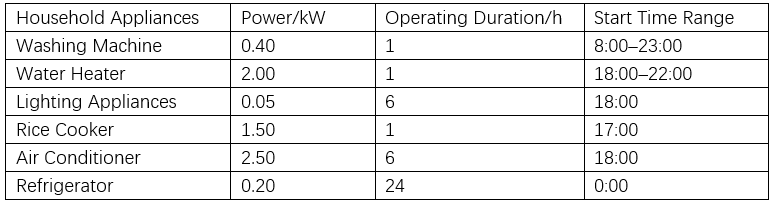
Set \(n = 144\), dividing the 24-hour day evenly into 144 time intervals, with each interval being 10 minutes. Figure 3 shows the power generation curve of the PV system on a certain day. The operation parameters of household loads are shown in Table 2, where the washing machine and water heater are shiftable loads.
Based on the above data in Table 2, Matlab is used to conduct a simulation study on the optimal management of household loads. According to the home energy efficiency management algorithm, the optimal household electricity usage scheme is determined to minimize the total daily electricity cost. The simulation results are shown in Figure 4.
After simulations, the minimum total household electricity cost occurs when \(T_{\text{Li1}} = 133\) and \(T_{\text{Li2}} = 132\) (washing machine starts at 22:00, water heater at 21:50).
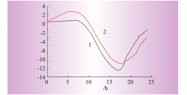
Figure 4 shows the daily cost curve. Curve 1 (no energy management) and Curve 2 (with load shifting and storage control) reveal: Negative costs mean grid-feed revenue + PV subsidies > grid costs. Post-6:00, PV growth cuts costs until 17:00 (PV drops to 0, grid supply raises costs), ending at \(C = -2.02\) CNY at 24:00.
With energy management, Curve 2 shows: Post-0:00, battery charging (from grid) boosts costs fast. Post-17:00, battery supply slows cost growth vs Curve 1. Load shifting further reduces costs, ending at \(C = -4.10\) CNY (a 2.08 CNY decrease). Simulations confirm the algorithm works—cutting costs, improving economy, and achieving peak-shaving.
5. Conclusions
A ZigBee-based smart home system integrating PV, storage, and energy management is designed. A mathematical model and time-of-use pricing-based algorithm are built. Simulations show it optimizes storage charging/discharging and load timing, slashing costs, boosting benefits, and proving feasibility.