Bayanin Muhaɗi na Makarfiyar Tattalin Nuna
Tattalin nuna ta yi amfani da mutanen tattalin nuna da kuma mutanen tattalin nuna. Makarfiyar tattalin nuna suna cikin hanyoyi masu tarihi na tattalin nuna. A cikin waɗannan makarfiya, anke da kasa, tattalin nuna mai yawa, gas, biyofuel, da kuma biogas zai gama a cikin tufafi.
Tufafin tattalin nuna wani hanyoyi mai yawa. Idan a fahimta, zaka iya kawo shi a matsayin wurin da suka fi sanya da dukwuka, inda abincin mai ruwa ke ci gaba. An haɓaka tattalin nuna a cikin tufafi, zai haɗa wannan ruwa. A cikin wannan inganci, ruwan ya zama asan steam mai tsarki (da tsarin kirkiro daga 150 ksc zuwa 380 ksc, idan bayan hanyoyin) da kuma mai tsari (daga 530°C zuwa 732°C, idan bayan hanyoyin).
Wannan asan steam ya zama zai haɗa a cikin turbine, inda ya zama da tsarki rarrabe da kuma tsari. A cikin wannan inganci, asan steam ya ba tattalin nuna da energy da take da. Maimaita asan steam a cikin turbine ya zama zai haɗa da yanayin turbine. Turbine ya zama zai haɗa da generator mai tsarki.
Generator mai tsarki ya zama zai haɗa da energy mai tsarki da turbine da ita. Generators mai tsarki suna ba da energy a tsari mai yawa, da kuma tsari mai yawa, typically in the range of 11 kV to 26 kV, at the nominal frequency. Wannan tsari ya zama zai haɗa a cikin generating transformer don samun karfin da zai haɗa a cikin grid. A cikin bincike da take da, wannan hanyoyi mai yawa ce ake kira shi a matsayin tattalin nuna.
Turbine Governor Control (TGC)
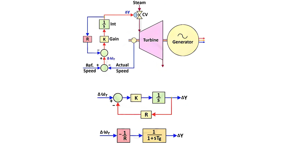
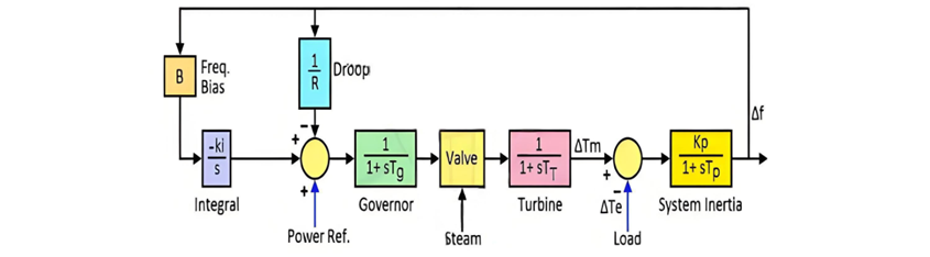
Kamar yadda ake bayyana, governor ya zama zai haɗa da maimaita asan steam a cikin turbine da ita. Governor hydraulic ya zama zai haɗa da feedback daga tsari mai yawa da turbine. Figure 1 ta bayyana yadda governor ya yi a cikin mode na tsari.
Tsari mai yawa da turbine ya zama zai haɗa da tsari mai yawa (da take da tsari mai yawa). Wannan tsari error signal (∆ωᵣ) ya zama zai haɗa a cikin governor. Daga baya, governor ya zama zai haɗa da maimaita valve: idan ana samu signal mai yawa (da take da tsari mai yawa), governor ya zama zai haɗa da valve; idan ana samu signal mai yawa, governor ya zama zai haɗa da valve.
“R” ta zama zai haɗa da setting na governor, typically ranging from 3% to 8%. Mathematically, it is defined as:
R = (per unit change in frequency) / (per unit change in power)
Droop settings are critical for the stable parallel operation of multiple generating units, as they determine how load is shared within a control area. Units with a smaller droop value will automatically assume a larger share of the load.
Control Area
In a power system, generating units and loads are distributed across vast geographical regions. To maintain stability, the entire grid is divided into smaller control areas (primarily based on geography). This division enables:
Within a control area, multiple generating units and loads coexist. Subdividing the power system into control areas serves several key objectives:
1. Load Frequency Control
This framework enables the application of load - frequency control methods to maintain grid frequency—a concept explored in greater detail later.
2. Determination of Scheduled Interchanges
If a control area’s generation falls short of its load demand, power flows into the area from neighboring control areas via tie lines (and vice versa).
3. Effective Load Sharing
Load demand varies throughout the day (e.g., lower at night, peaking in the morning and evening). Control areas simplify the process of:
Power Balance
Electrical energy is consumed in real - time (it cannot be stored on a large scale). Thus, power balance is a fundamental requirement:
Power Generated (P₉) = Load Demand (Pd) + Transmission Losses (Pₗ)
Transmission losses typically account for ~2% of generated power and are often neglected when focusing on frequency control. For simplicity, we approximate:
Power Generated (P₉) ≈ Load Demand (Pd)
Frequency Variation
Grid frequency fluctuates due to mismatches between load demand and generation. While minor deviations are stabilized by system inertia, significant gaps (e.g., unit trips, large load changes) can cause frequency to vary by ±5%. Key scenarios include:
In most cases (e.g., unit/line trips, large load connection), demand exceeds generation, causing frequency to drop. Conversely, if a transmission line serving a large load trips, generation may exceed demand, causing frequency to rise. Though the system responds oppositely to these scenarios, understanding frequency dips suffices to grasp both behaviors.
Why Frequency Dips Occur
Two inherent system behaviors drive frequency dips:
1. Load Dampening
Induction motors (e.g., household fans, industrial drives) dominate grid loads. Their power consumption is frequency - dependent: a 1% frequency reduction typically reduces active power consumption by ~2% in large systems. When new loads connect, frequency drops, and existing induction loads automatically consume less power—partially mitigating the demand - generation gap.
2. Kinetic Energy Release from Turbine - Generator (TG) Sets
Conventional TG sets have massive rotors (often >25 tonnes) spinning at 3000 RPM (for 50Hz grids). When demand exceeds generation, these rotors temporarily supply stored kinetic energy (for 3–5 seconds, depending on inertia). As rotors slow down, grid frequency drops.
Frequency Control
Load - frequency control (LFC) restores grid frequency to its nominal value after demand - generation mismatches. Two tiers of control exist:
1. Primary Frequency Control
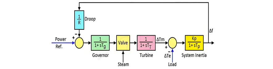
At the unit level, the turbine’s governing system adjusts speed (and thus frequency). As shown earlier, each unit modulates steam input based on frequency deviations. The full primary control loop for a generating station is depicted in the figure below.
2. Secondary Frequency Control
This involves coordinated control across multiple units in different control areas, ensuring long - term frequency stability and optimal load sharing.
Primary Frequency Control Limitations
Primary frequency control alone results in a steady - state frequency deviation, influenced by the governor droop characteristic and load frequency sensitivity. This occurs because individual units adjust speed without considering where new loads are connected or how much load is added. Without such contextual assessment, power balance cannot be fully restored, and frequency deviation persists. Following primary control actions, the steady - state frequency error may be either positive or negative.
Secondary Frequency Control
Restoring system frequency to its nominal value requires secondary control, which accounts for new load locations and adjusts reference setpoints for selected units. When load increases in a control area, generation within that area must rise to:
To achieve this:
Once revised load setpoints are issued, units begin adjusting generation. Due to the mechanical nature of power production, it takes 25–30 minutes for units to reach their scheduled outputs. When all generating stations achieve target generation, power balance is reinstated, and frequency returns to nominal.
The overall response of the system with the primary and secondary frequency control can be understood by the graph below.
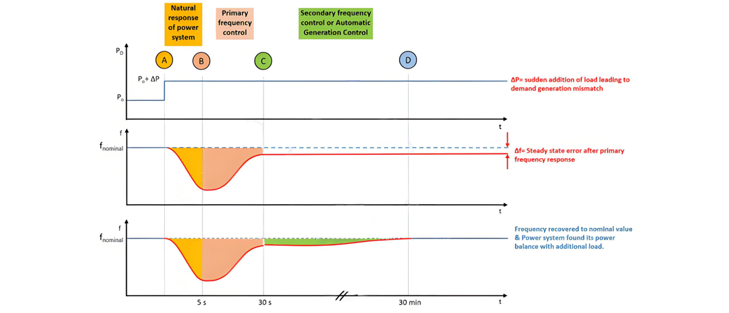
System Response to Load Increase (A-B-C-D)
A-B: Transient Kinetic Energy Release
Before point A, the system operates in power balance. At point A, load suddenly increases from P₀ to P₀ + ∆P. A 3–5 second delay occurs before the governor responds. During this interval, the rotor's stored kinetic energy supplies the excess load, causing rotor speed to drop and frequency to dip to a minimum value f₁.
B-C: Primary Frequency Control Action
At ~5 seconds, the governor initiates speed control, increasing steam input to restore rotor speed. This phase lasts 20–25 seconds (dependent on the frequency dip magnitude). As discussed, primary control alone leaves a steady - state frequency error ∆f due to governor droop.
C-D: Secondary Frequency Control (AGC Activation)
Once frequency stabilizes, secondary control (via AGC) adjusts generation for selected units in each control area. This process considers:
Generation adjustments are limited by the units’ design ramp rates, taking several minutes to complete. Upon finishing, scheduled interchanges return to pre - calculated values, and the system achieves a new power balance with nominal frequency.