The order of a control system is determined by the power of ‘s’ in the denominator of its transfer function.
If the power of s in the denominator of the transfer function of a control system is 2, then the system is said to be second order control system.
The general expression of the transfer function of a second order control system is given as
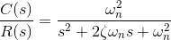
Here, ζ and ωn are the damping ratio and natural frequency of the system, respectively (we will learn about these two terms in detail later on).
Rearranging the formula above, the output of the system is given as
If we consider a unit step function as the input of the system, then the output equation of the system can be rewritten as

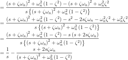

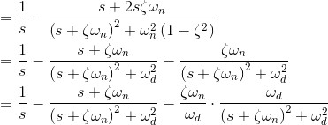
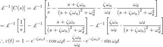
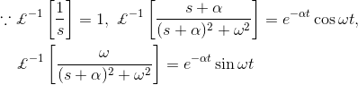
Taking the inverse Laplace transform of above equation, we get
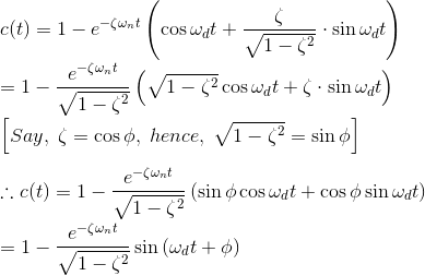
The above expression of output c(t) can be rewritten as
The error of the signal of the response is given by e(t) = r (t) – c(t), and hence.

From the above expression it is clear that the error of the signal is of oscillation type with exponentially decaying magnitude when ζ < 1.
The frequency of the oscillation is ωd and the time constant of exponential decay is 1/ζωn.
Where, ωd, is referred as damped frequency of the oscillation, and ωn is natural frequency of the oscillation. The term ζ affects that damping a lot and hence this term is called damping ratio.
There will be different behaviors of output signal, depending upon the value of damping ratio and let us examine each of the cases, one by one.
Using this as a base, we will analyze the time response of a second order control system. We’ll do this by analyzing the unit step response of a second order control system in the frequency domain, before converting it into the time domain.
Step Response of Second Order System
When damping ratio is zero, we can rewrite the above expression of output signal as

As in this expression, there is no exponential term, the time response of the control system is un-damped for unit step input function with zero damping ratio.
Page 137. Figure 6.4.3. of the book automatic control system by Hasan.
Now let us examine the case when damping ratio is unity.
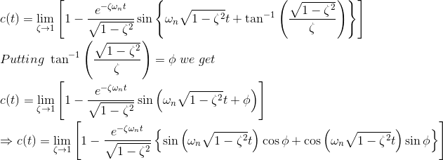
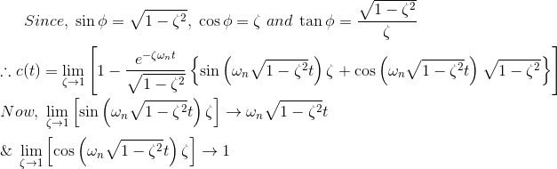

In this expression of output signal, there is no oscillating part in subjective unit step function. And hence this time response of second-order control system is referred as critically damped.
Now we will examine the time response of a second order control system subjective unit step input function when damping ratio is greater than one.
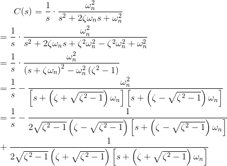
Taking inverse Laplace transform of both sides of the above equation we get,


In the above expression, there are two time constants.
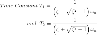
For the value of ζ comparatively much greater than one, the effect of faster time constant on the time response can be neglected and the time response expression finally comes as
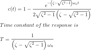
Figure 6.4.5 of the page 139 of the book automatic control system by Hasan.
Critical Damping Time Response of Control System
The time response expression of a second order control system subject to unit step input function is given below.

The reciprocal of constant of negative power of exponential term in the error part of the output signal is actually responsible for damping of the output response.
Here in this equation it is ζωn. The reciprocal of constant of negative power of exponential term in error signal is known as time constant.
We have already examined that when the value of ζ (also know as damping ratio) is less than unity, the oscillation of the response decays exponentially with a time constant 1/ζωn. This is called under damped response.
On the other hand. when ζ is greater than unity, the response of the unit step input given to the system, does not exhibit oscillating part in it.
This is called over damped response. We have also examined the situation when damping ratio is unity that is ζ = 1.
In that situation the damping of the response is governed by the natural frequency ωn only. The actual damping at that condition is known as critical damping of the response.
As we have already seen in the associated expressions of time response of control system subject to input step function, the oscillation part is present in the response when damping ratio (ζ) is less than one and it is not present in the response when damping ratio is equal to one.
That means the oscillation part of the response just disappears when the damping ratio becomes unity. That is why damping of the response at ζ = 1, is known as critical damping.
More precisely, when damping ratio is unity, the response is critically damped and then the damping is known as critical damping.
The ratio of time constant of critical damping to that of actual damping is known as damping ratio. As the time constant of time response of control system is 1/ζωn when ζ≠ 1 and time constant is 1/ωn when ζ = 1.

Second Order System Transfer Function
The general equation for the transfer function of a second order control system is given as

If the denominator of the expression is zero,
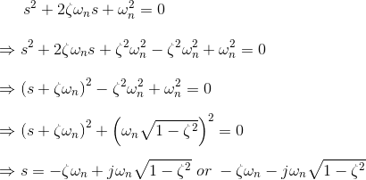
These two roots of the equation or these two values of s represent the poles of the transfer function of that system. The real part of the roots represents the damping and imaginary part represents damped frequency of the response.
The location of the roots of the characteristics equation for various values of ζ keeping ωn fixed and the corresponding time response for a second order control system is shown in the figure below.
Figure 8.4.7 page 140 of the book automatic control system by Hasan.
Transient response specifications of second-order control system.
The performance of the control system can be expressed in the term of transient response to a unit step input function because it is easy to generate.
Let us consider a second-order control system in which a unit step input signal is given and it is also considered that the system is initially at rest. That is all initial conditions of the system are zero. The time response characteristics of the system at under damped condition is drawn below.
Figure 2.17 page 92 of the book automatic control system by Hasan.
There are number of common terms in transient response characteristics and which are
Delay time (td) is the time required to reach at 50% of its final value by a time response signal during its first cycle of oscillation.
Rise time (tr) is the time required to reach at final value by a under damped time response signal during its first cycle of oscillation. If the signal is over damped, then rise time is counted as the time required by the response to rise from 10% to 90% of its final value.
Peak time (tp) is simply the time required by response to reach its first peak i.e. the peak of first cycle of oscillation, or first overshoot.
Maximum overshoot (Mp) is straight way difference between the magnitude of the highest peak of time response and magnitude of its steady state. Maximum overshoot is expressed in term of percentage of steady-state value of the response. As the first peak of response is normally maximum in magnitude, maximum overshoot is simply normalized difference between first peak and steady-state value of a response.

Settling time (ts) is the time required for a response to become steady. It is defined as the time required by the response to reach and steady within specified range of 2 % to 5 % of its final value.
Steady-state error (e ss ) is the difference between actual output and desired output at the infinite range of time.

Rise Time Formula
The expression of under damped second-order control system with unit step input function,

Again, as per definition, the magnitude of output signal at Rice times is 1. That is c(t) = 1, hence

Peak Time Formula
As per definition at the peak time, the response curve reaches to its maximum value. Hence at that point,

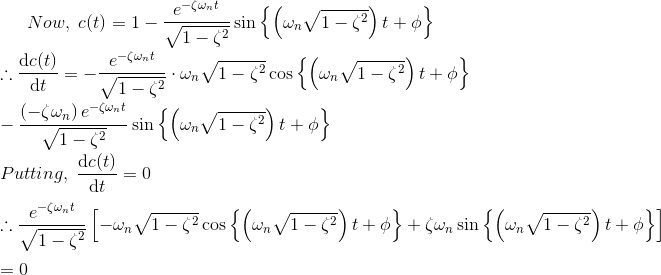
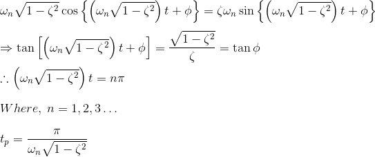
The maximum overshoot occurs at n = 1.
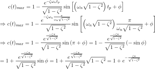
Maximum Overshoot Formula
If we put the expression of peak time in the expression of output response c(t), we get,

Settling Time Formula
It is already defined that settling time of a response is that time after which the response reaches to its steady-state condition with value above nearly 98% of its final value.
It is also observed that this duration is approximately 4 times of time constant of a signal. At the time constant of a second-order control system is 1/ζ ωn, the expiration of settling time can be given as
 Statement: Respect the original, good articles worth sharing, if there is infringement please contact delete.

 Login